Tutorial roadmap
We start with the adaptation options, then cover evaluation, then walk through the XRD notebook examples and results.
Foundation models and adaptation
choose what to change
Evaluation is part of the method
know whether it worked
XRD example
compare the notebook results
Foundation models and how to adapt them
Start with the simplest method that can answer your question. Add complexity only when the evidence calls for it.
Where foundation models fit in
Foundation models are deep-learning models trained broadly once, then adapted many times for specific tasks.
What foundation models can do
A pretrained model can help with routine analysis, natural-language interfaces, and discovery workflows when the task is well defined.
Automate routine tasks
Summarize, classify, extract, write code, and check repeated analysis steps.
Create natural interfaces
Let scientists ask for analysis, metadata, and visual explanations in normal language.
Accelerate discovery
Combine search, simulation, and experiment loops around measured outputs.
Pretraining is done once. Adaptation happens in the lab.
Model providers usually handle broad pretraining. Scientific users decide how the model is adapted, tested, and used.
model learns broad patterns from large datasets
choose prompts, examples, features, or adapters
use only after behavior has been measured
- Domain mismatch
- Hallucinations
- Hidden failure modes
- Benchmark first
- Adapt if needed
- Scaffold with workflows
The adaptation landscape
This map compares strategies by how much they change the input, how much they change the model, and how much work they require.
Zero-shot
jump to sectionDescribe the task and ask the model. Model weights do not change. Useful as a baseline even when you expect it to fail.
- labels
- 0
- compute
- API or local CPU
- iteration
- seconds
- fast triage
- format testing
- early prototyping
- unstable formats
- hallucinated labels
- weaker domain grounding
Click a strategy to compare its costs. More expensive is not automatically better: move to heavier methods only when simpler ones stop making real progress.
Compute and memory trade-offs
Labels, compute, and iteration time change quickly as you move from prompting to adapters and full fine-tuning.
Strategy 0: zero-shot prompting
A good prompt states the task, goal, context, and constraints clearly. Start simple before adding fragile prompt tricks.
Given this diffraction image, identify every anomaly that applies.
What should the model do?
What counts as a useful answer?
What domain facts or label definitions matter?
What constraints, units, or format should be respected?
- Fast triage
- Format testing
- Early prototyping
- Unstable formats
- Hallucinated labels
- Weaker domain grounding
Ask for structured outputs
For automation, the answer needs to be easy to parse and check. A schema helps downstream code trust what it receives.
response_format={"type": "json_object"}
{
"wavelength_A": 0.9763,
"detector_distance_mm": 250.0,
"beam_center_px": [1024, 1024],
"exposure_s": 0.5
}Simple and low-boilerplate, but you still need to validate the fields.
class XRDMetadata(BaseModel):
wavelength_A: float
detector_distance_mm: float
beam_center_px: tuple[int, int]
exposure_s: float | None = None
response_format=XRDMetadataMore setup, but the response is easier to check and use in Python.
Few-shot prompting
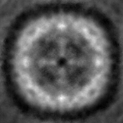
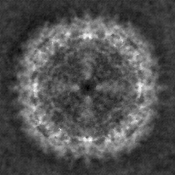
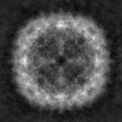
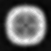
Few-shot prompting puts worked examples in the prompt. The model weights do not change.
- Allowed label set
- Expected answer format
- Multi-label edge cases
- A model that cannot read the pattern
- Data leakage
- An evaluation split that does not match the task
Frozen features
A scientific image becomes an embedding vector. A small classifier then works on those saved vectors.
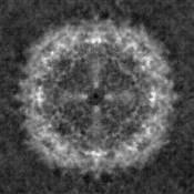
- Numeric summary of an image
- Similar images should be nearby
- The classifier learns from vectors instead of raw pixels
- Run the pretrained encoder once
- Save one vector per image
- Train a small head on vectors + labels
- Evaluate with the same split
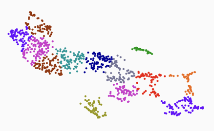
Example clustering of embeddings
If the encoder is useful, visually similar diffraction patterns should sit near one another in embedding space.
kNN vs. linear probe
Both methods use the same saved embeddings. kNN predicts from nearby examples; a linear probe learns a simple boundary.
Both methods read the same embedding. kNN votes with the 5 nearest labeled points; the linear probe only checks which side of its boundary you are on. Try the pocket of anomalous points at the bottom left: kNN follows the local labels, the linear probe cannot.
Move toward the boundary, or into the bottom-left pocket, to find where the two rules split.
- Sensitive to noisy labels
- Needs similarity search at inference
- Does not give calibrated probabilities by default
- Needs enough examples per class
- Must be re-fit when labels change
- Does not show similar examples by itself
LoRA fine-tuning
LoRA keeps most model weights fixed and learns a small low-rank update for the task.
- Full fine-tune: update all weights
- LoRA: train adapter matrices
- QLoRA: quantized base plus LoRA adapters
- Rank controls adapter size
- Typical r = 8-32
- Larger r adds flexibility and overfit risk
- Swap adapters without replacing the base model
- Each task can have its own adapter
- QLoRA stores the base in 4-bit and trains adapters in float16
Fine-tuning tools
There are many post-training methods beyond this tutorial. Open-source tools make them practical enough to try.
These tools make experiments easier to run, but they do not replace clean splits, metrics, and ablations.
Evaluation is part of the method
A model result is only useful if the evaluation matches the scientific question.
Train, validation, test - and why it matters
Use training for fitting, validation for choices, and test once for reporting. Split by physical object when related images could leak information.
fit parameters
choose thresholds and settings
report once
Training loss can keep improving while validation loss turns upward. Report the held-out test result after model choices are finished.
Confusion matrices and F1
Precision, recall, and F1 all come from the same four counts. Choose the metric that matches the scientific cost of mistakes.
Drag the threshold. Coral dots are mistakes: positives that fall below it (FN) and negatives that clear it (FP). Every metric on the right is just a different way of counting them.
predicted +, actually +
predicted +, actually -
predicted -, actually +
predicted -, actually -
Multi-label metrics: micro-F1 and macro-F1
Micro-F1 pools all decisions. Macro-F1 makes rare labels visible.
The two common labels stay fixed. Only the rare label degrades, and the two averages tell very different stories about it.
Pools all decisions first. Frequent labels dominate, so it barely notices the rare label failing.
Averages per-label scores. The rare label carries a full third of the weight, so its failure is visible.
Non-classification metrics
Use the lightest evaluator that can catch the failure: schema checks, runnable tests, reference answers, grounding checks, or judges.
Use schema checks and parsers.
Run unit tests, examples, and integration tests.
Compare against reference outputs.
Check grounding, retrieval, and source coverage.
Use rubrics, human review, or LLM judges as a last layer.
The XRD example
A public diffraction dataset, three notebooks, and a reminder to measure before adding complexity.
The public dataset
The RefleX dataset has 6,311 diffraction images, seven anomaly labels, official splits, and many images with more than one anomaly.
The task: multi-label XRD anomaly detection
Input one diffraction image. Return every anomaly label that applies.

Preparing scientific images for foundation models
Dynamic range choices matter. The training and inference preprocessing should be the same.

clip, log-scale, normalize
use the same transform for training and inference
- Detector counts span orders of magnitude
- Raw values can exceed 10,000
- Natural-image encoders expect different image statistics
- Convert 16-bit detector images before modeling
- Use a fixed range for comparability
- Percentile normalization can reduce outlier effects
- Use log10(x + epsilon) when needed
- Compress bright peaks
- Expose weak features humans inspect
Notebook 1: few-shot prompting
Send diffraction images and text examples in the prompt. The model weights never change.

- Prompt design
- Output parsing
- Effect of adding support examples
- Set OPENAI_API_KEY before running
Random support examples can miss important labels. A stronger version would choose examples by similarity and label balance.
Notebook 2: frozen features + light classifier
Encode the images once with CLIP, then fit kNN or a linear classifier on the embeddings.

- Frozen CLIP ViT-L/14-336 encoder
- Mean-max pooled patch-token embeddings
- Heads: kNN, one-vs-rest logistic regression, low-shot logistic regression
- The encoder is reused rather than retrained
0.819 macro-F1 on full RefleX test set
0.789 macro-F1 with validation-tuned threshold
Notebook 3: LoRA fine-tuning of Gemma 3 4B
Fine-tune Gemma 3 4B with QLoRA, PEFT, and TRL. In this run, extra few-shot examples hurt after SFT.

- LoRA r=16, alpha=16, dropout 0.05
- 1 epoch, lr 2e-4, gradient accumulation 4, MAX_SOFT_TOKENS=280
- Accept the model terms before downloading
- A free-tier T4 GPU is not enough for this run
After SFT, extra in-context examples made this run worse. Measure the adapted model both with and without examples.
Simpler methods can be better
On this benchmark, frozen CLIP plus kNN is simpler and stronger than the more complex alternatives tested here.
SFT and few-shot may not help each other
Prompting and fine-tuning do not automatically combine well. Test the combined setup before relying on it.
Glossary
Key terms from the tutorial, related ptychography references, and acknowledgements.
Glossary
A quick reference for the main terms used above.
Ask the model directly, no worked examples.
Include a handful of worked examples in the prompt.
A numeric summary of an image or text.
The model part that turns input into a representation.
Predict from the most similar labeled examples.
A simple rule drawn in feature space.
Updating model weights on your task.
A small trainable add-on instead of full retraining.
Lower-precision storage to save memory.
Related samples in train and test that inflate scores beyond real-world performance.
Pool-then-score (micro) vs. score-then-average across classes (macro).
Supervised fine-tuning on labeled input–output pairs.
LoRA on a quantized base model, often small enough for a single GPU.
Out-of-distribution: inputs unlike what the model trained on.
For ptychography examples beyond this XRD tutorial, see arXiv:2511.02503 and arXiv:2410.09034, which show how LLMs and VLMs can be adapted to ptychography tasks and how agentic workflows can be built around tested model recipes.
Acknowledgement: this research used resources of the Advanced Photon Source, a U.S. DOE Office of Science User Facility operated under Contract DE-AC02-06CH11357, with funding support from Argonne LDRD 2023-0049. Thanks to APS MIC/CAI/SDM groups, USC Shao Group, Rice Han Group, and Cornell Muller Group.